Satellite images for irrigation: what NDVI and thermal data can and cannot tell a farmer
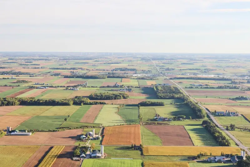
Photo: rawpixel (CC0, credits)
Free satellite imagery now covers almost every irrigated field on Earth every few days. Services sell it as a map of “water stress”, an NDVI layer or an evapotranspiration estimate. Behind those products are two quite different measurements: how green and dense the crop is, and how warm its surface is. Knowing which one a service relies on tells an irrigator what the map can answer and what it cannot.
Two things a satellite can measure
Optical satellites record the sunlight reflected by the ground in several wavelength bands. Healthy leaves absorb most red light for photosynthesis and reflect strongly in the near infrared, because of the internal structure of the leaf. Bare soil reflects the two more evenly. The contrast between red and near-infrared reflectance is therefore a good proxy for how much green canopy covers the ground.
Thermal sensors measure something else: the temperature of the surface. A crop that transpires freely is cooled by the evaporation of water from its leaves, much as sweating cools the skin. When water runs short, the stomata close, transpiration falls and the canopy warms up. Temperature reacts to water stress within days or even hours; greenness reacts only once growth has already been affected.
The first kind of measurement describes the crop's size, the second its current water use. Most irrigation products combine one or both with the weather-based calculation explained in our article on crop evapotranspiration and FAO-56.
Vegetation indices and the crop coefficient
The most common index, NDVI (normalised difference vegetation index), is the difference between near-infrared and red reflectance divided by their sum. It runs from around zero over bare soil to values approaching 0.9 over a dense, healthy canopy. The formula was proposed by Rouse and colleagues in 1974, for the first Landsat satellite, and has been used in agriculture ever since. Variants such as SAVI correct for the influence of bright soil showing between rows, which matters in young orchards and vineyards.
For irrigation scheduling, the useful link is between ground cover and the crop coefficient, Kc. FAO-56 tabulates coefficients for a healthy crop with full cover. Real fields differ: a young orchard, a patchy stand or a crop sown late uses less water than the table assumes. In 2009, Richard Allen and Luis Pereira published a method to estimate the basal crop coefficient from the fraction of ground covered by vegetation and the height of the crop, so that the coefficient follows the real canopy rather than a generic curve (Allen and Pereira, Irrigation Science, 2009). Ground cover can be measured in the field, from photographs, or estimated from a vegetation index, which is how satellite images enter the calculation.
The practical result is a Kc map, updated each time a clear image arrives. Multiplied by the reference evapotranspiration from a nearby weather station, it gives an estimate of crop water use field by field, or zone by zone inside a field. This is exactly the correction the FIGARO partners had in mind when they described canopy sensors and satellite images as a way to keep crop models in step with what grows in the field (see sensors and satellite images in precision irrigation).
The limit is built into the method. A vegetation index describes how much canopy there is, not whether that canopy is short of water today. A well-irrigated field and a field entering stress look the same in NDVI for days. By the time stress shows as reduced greenness, part of the yield may already be lost. Index-based coefficients are therefore best for how much water a crop needs over the coming week, not for detecting a failed irrigation.
Thermal imagery and energy balance models
Thermal data allow a more direct estimate. Energy balance models treat evapotranspiration as what is left of the energy the surface receives: net radiation, minus the heat that goes into the soil, minus the heat that warms the air. The warmer the surface compared with the air, the more energy goes into heating and the less into evaporating water.
Two models of this family are widely used. SEBAL was developed by Wim Bastiaanssen and colleagues in the 1990s. METRIC, published by Allen, Tasumi and Trezza in 2007 in the Journal of Irrigation and Drainage Engineering, adapted it for irrigated agriculture. Both calibrate each image internally with two reference pixels chosen by the analyst or an algorithm: a “cold” one, a well-watered full crop transpiring at its maximum, and a “hot” one, dry bare soil with almost no evaporation. Every other pixel is placed between these extremes. The approach avoids the need for precise absolute temperature calibration, but makes the result depend on finding good reference pixels in each scene.
The output is an actual evapotranspiration map, reflecting stress if there is any. It shows the field that is not getting enough water, and also the one getting too much, where nothing limits evaporation but the drainage losses are invisible. Public programmes now publish such estimates routinely: FAO's WaPOR portal on water productivity, and the OpenET consortium for the western United States, both derived from satellite data and freely accessible.
Pixels, revisits and clouds
Whether these products can steer a particular field depends on three practical constraints.
| Constraint | Optical (e.g. Sentinel-2) | Thermal (e.g. Landsat) |
|---|---|---|
| Pixel size | 10 m for the red and near-infrared bands | Coarser: thermal bands are acquired at about 100 m and resampled |
| Revisit | Every 5 days at the equator with two satellites, more often at higher latitudes | About every 8 days with two satellites |
| Clouds | No usable data under cloud | No usable data under cloud |
| Best use | Ground cover, crop coefficient, variability inside a field | Actual evapotranspiration, stress, comparison between fields |
The Sentinel-2 figures come from the mission description published by the Copernicus programme, which gives 13 spectral bands, four of them at 10 m resolution, and a 290 km swath (Sentinel-2 mission overview). A 10 m pixel is fine for a maize field or a citrus block; for narrow vegetable beds or individual trees, each pixel mixes canopy, soil and sometimes the drip line's wet strip. A 100 m thermal pixel, even when sharpened, mostly describes whole fields.
Clouds are the hardest limit. In a wet spring, there may be no clear image for weeks, precisely when crops establish. Products fill the gaps by interpolating between clear dates, which is reasonable for slowly changing ground cover and much less so for stress. Some services add radar, which sees through clouds and responds to surface moisture and canopy structure, but its signal is harder to interpret in terms of crop water use.
How to use satellite data well
- Ask what the map is. NDVI, crop coefficient and actual evapotranspiration answer different questions. A “stress map” built only from greenness is a growth map.
- Check the date of the last clear image. A map interpolated from an image ten days old says little about this week.
- Use it to find patterns, then go and look. A persistently weak strip along a lateral often points to a hydraulic problem. Our article on drip irrigation uniformity explains how to measure it on the ground.
- Combine it with point measurements. A satellite sees the whole field but not the root zone; a probe sees the root zone at one spot. Satellite maps are a good guide for choosing where to install the soil moisture sensors and for checking whether their spot is representative.
Used this way, satellite images do not replace the water balance or the probes. They extend both to the whole farm, at almost no cost, and show where a schedule calculated for an average field does not fit the field that actually grows.
Sources
- Allen R. G., Pereira L. S. (2009), “Estimating crop coefficients from fraction of ground cover and height”, Irrigation Science 28(1): 17–34.
- Allen R. G., Tasumi M., Trezza R. (2007), “Satellite-based energy balance for mapping evapotranspiration with internalized calibration (METRIC): model”, Journal of Irrigation and Drainage Engineering 133(4): 380–394.
- Copernicus / European Space Agency, Sentinel-2 mission overview, SentiWiki.
- Rouse J. W., Haas R. H., Schell J. A., Deering D. W. (1974), “Monitoring vegetation systems in the Great Plains with ERTS”, Third ERTS Symposium, NASA SP-351, vol. 1, pp. 309–317.